Understanding Transmission Line Losses in High-Speed Signals

In surveying the subject of debugging high-speed serial data links, we've noted that there's no one cause for signal-integrity issues between transmitter and receiver, and there's certainly no one solution. But let's begin with the low-hanging fruit: electrical losses in the transmission line. We've previously done a series of posts on transmission lines (beginning here), but it's worth it to have a quick refresher.

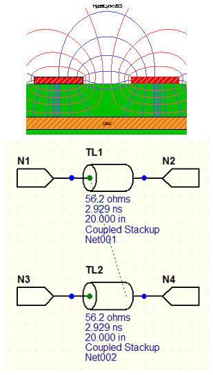
Figure 1 depicts a 20-inch-long, FR-4 microstrip differential trace as simulated using a 3D field solver. There is a spacing of 5 mils between the P and N lines, which themselves are 5 mils wide. With one channel width worth of spacing between them, the two lines are rather tightly coupled to each other.

An advantage of using a 3D field solver is the ability to visualize the field lines on the dielectric and from the conductors themselves. This gives you some insight into the coupling and of the field transmission along the traces. The schematic renderings of Figure 1 show a single-ended impedance of 56.2 Ω for the traces, which is a non-ideal impedance. But it also implies that the differential impedance is about 100 Ω.

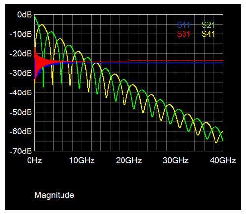
A look at the single-ended parameters (Figure 2) reveals ringing due to the dips in the insertion loss and return loss. However, the mixed-mode parameters (Figure 3) are essentially flat, due to that differential impedance of about 100 Ω. The single-ended impedance is a little higher than that because of the coupling effects.

For transmission lines of this nature carrying serial data at very high rates, the primary signal-loss mechanisms are skin effect and dielectric losses. Skin depth is inversely proportional to the signal's frequency, so the higher we go in frequency, the less deeply the current penetrates into the conductor. Rather, it remains on the conductor's surface, which increases resistance and radiation losses at these higher frequencies.

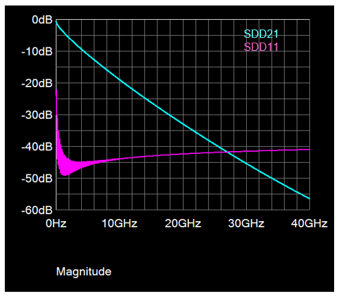
Further, dielectric losses include the effects of loss tangent and dielectric conductivity. All of these contribute to higher losses at higher frequencies, which is quite evident in the plot of losses shown in Figure 3. Beyond 10 GHz or so, the losses are significant and will lead to degraded eye performance at the receiver.

In another post, we'll continue looking at these loss mechanisms and address the elephant in the room: How much loss is too much?

Copyright © 2020-2026 Teledyne LeCroy. All rights reserved. All original content, including text and photos, is the property of Teledyne LeCroy and cannot be reproduced without expressed written permission.