Radar Signal Analysis With Oscilloscope Demodulation
Learn how oscilloscope demodulation and FFTs reveal radar pulse envelopes, Barker-coded phase modulation, chirp behavior, and frequency content.
Learn how oscilloscope demodulation and FFTs reveal radar pulse envelopes, Barker-coded phase modulation, chirp behavior, and frequency content.

This article explains the expected behavior of on-die power rails during CMOS switching events, including PDN current flow, clock-edge noise, and asymmetric current draw between switching and latching operations.

Learn how oscilloscope histograms help characterize component specifications by comparing propagation delay, mean, standard deviation, and measurement spread under different conditions.

This tutorial explains a robust oscilloscope-based method for measuring clock jitter using period statistics, track and histogram analysis, and sample-rate verification techniques.

Clock jitter is the variation of a clock signal’s frequency or period. Either measurement carries the same information, but the period measurement is a simple time interval measurement easily performed using a real-time oscilloscope. If we have a robust way of measuring clock jitter, we have the basis for measuring the clock signal’s sensitivity to other features in the environment that can affect the period. Voltage noise on the power rail is just one external force that can affect clock jitter, which we'll show you how to measure in a future post.
In this post, we’ll demonstrate a robust method for measuring clock jitter using an example from Dr. Eric Bogatin’s webinar, The Impact of Power Rail Noise on Clock Jitter.
The clock in our examples is a 5-stage ring oscillator which generates a square wave signal between 10 and 66 MHz. The test instrument is a WavePro HD 12-bit, 4-Ch, 8 GHz, 20 GS/s, 5 Gpts oscilloscope with 60 fs sample clock jitter.
In the process, we make a series of oscilloscope sample clock tests and timebase adjustments as consistency checks. While measuring jitter is less about absolute accuracy than about the relative precision of measuring the time interval from cycle to cycle, a fundamental part of that is ensuring the absolute accuracy of the oscilloscope’s timebase.
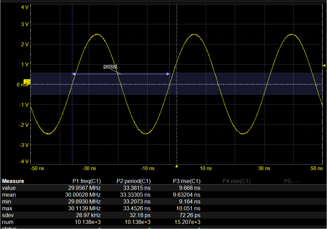
Before measuring the clock signal jitter, it’s advisable to do a “situational awareness” test of the oscilloscope’s timebase accuracy using a known source to verify it meets the specification. To do this, we use a synthesized function generator with 1 PPM absolute accuracy to generate a 30 MHz, 5V signal and apply it to the oscilloscope on C1. We set a 50% Edge trigger and a fixed sample rate of 20 GS/s (Figure 2). After measuring the known source frequency, rise time and period using parameters, we calculate the fractional uncertainty in PPM using the formula: (Δf/f)10^6. With a mean frequency of 30.00028 MHz, Δf =280 Hz, so the fractional uncertainty in PPM on a 30 MHz signal is 280/3010^6 = 9.333, indicating the absolute accuracy of the oscilloscope timebase is under 10 PPM. Pretty good.
Next, we switch the trigger to the clock source channel, and adjust the V/div and Time/div until two periods of the signal are visible on the graticule. Figure 3 shows the waveform of the ring oscillator on C2. The period is a little more than four divisions, which at 5 ns/division is about 21 ns. The rise time is a little less than two minor divisions, each of which represents 1 ns, so about 1.5 ns.
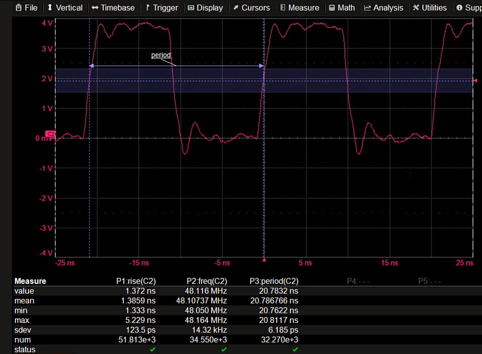
Using parameters with statistics on, we measure the rise time, frequency and period of the clock signal. The mean frequency is 48 MHz, corresponding to a period of 20.75 ns, very close to the estimated 21 ns, and within the specified 10 to 66 MHz. The estimated rise time was 1.5 ns, and the measured value is 1.38 ns.
The standard deviation (sdev) is a measure of the spread of values about the mean. By definition, in a Gaussian distribution, 68% of all measured values are within ±1 standard deviation from the mean. The period sdev value is a good figure of merit for clock jitter, which is a measure of variation from the mean.
With statistics on, the sdev of every parameter measurement is already calculated. Our clock period sdev measurement is 6.18 ps. However, since the oscilloscope’s intrinsic sample clock jitter is specified at 60 fs, and we have ascertained an accuracy of ~9 PPM, the measured period jitter at 6.18 ps is much higher than the fundamental limit of the oscilloscope. The measurement is likely “real.”
Keeping the maximum fixed sample rate, we increase the Time/div to 20 µs/div for a total acquisition time of 200 µs and record length of 4M sample points. At 4M points per acquisition and over 6.3 million measurements in the buffer, our period measurement still has an sdev of 6.1 ps— around 6 ps every 20 ns period, or about 0.03% variation in the period. (Figure 4).
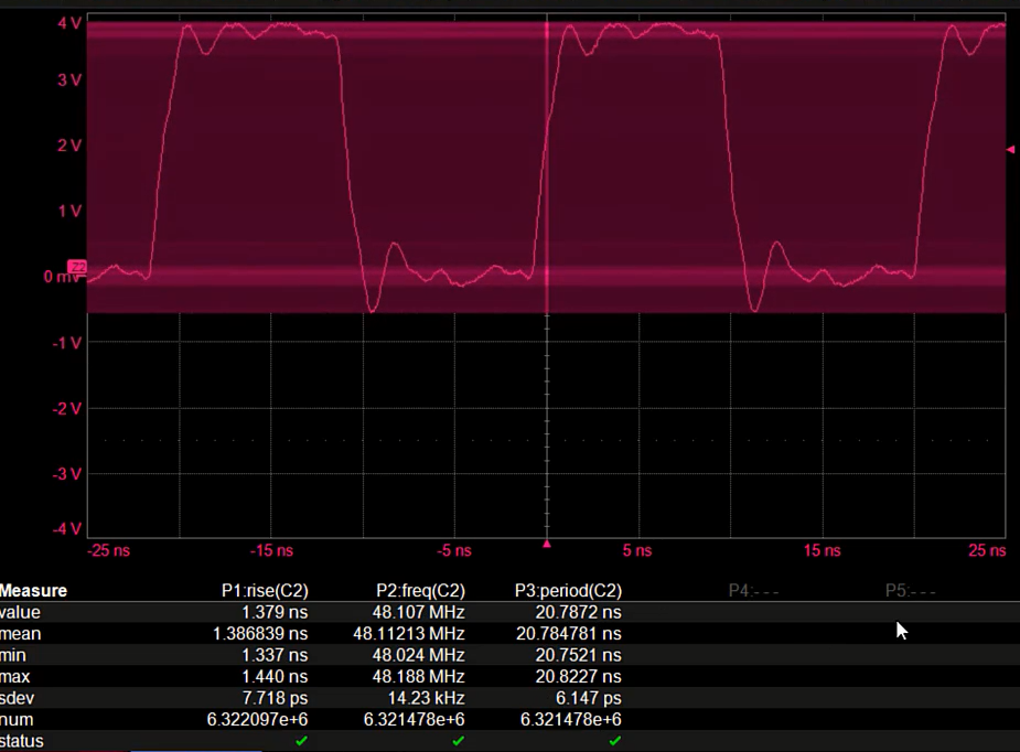
Figure 5 shows both the track and the histogram of our period measurement. The track function is displayed over the acquired waveform, while the histogram is plotted in a separate grid.
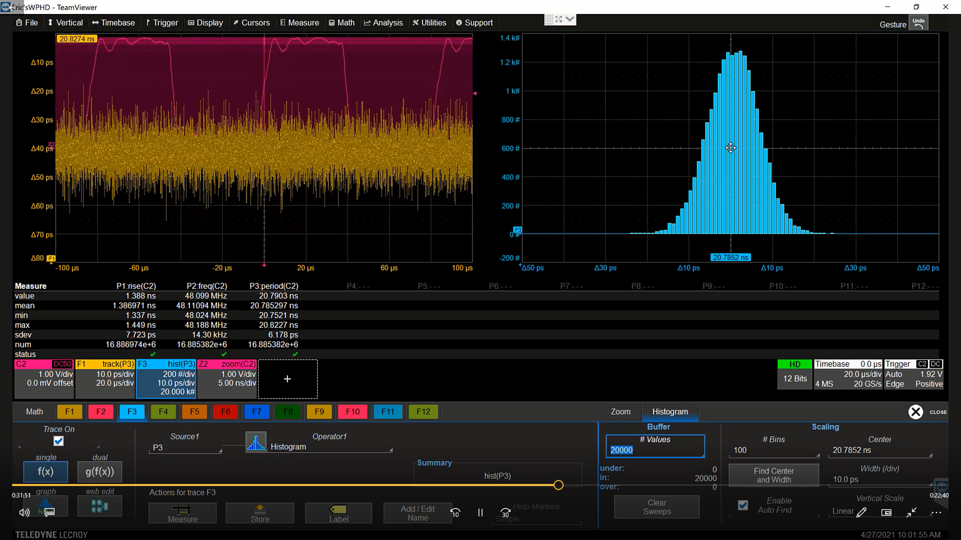
The vertical scale of our track function is 10 ps/div, same as the horizontal scale of our histogram. Just by “eyeballing” the extent of the track, we can confirm the sdev matches the 6 ps sdev that is calculated by the period measurement statistics. The histogram is centered near the mean value of the period measurement at 20.7852 ns. The saddle shape of the histogram is characteristic of the Gaussian or Normal distribution, a good indication that the clock jitter is the result of a random process.
As a consistency check, we investigate how the oscilloscope’s sampling rate affects the measured clock jitter. This is done for “situational awareness,” to ensure that the instrumentation is not affecting the measurements. We lower the sample rate by successive steps until the measurement visibly degrades. From 20 GS/s, we step to 10 GS/s, 5 GS/s and 2.5 GS/s with little change in the measured period sdev or the shape of the histogram. Only when we reach 1 GS/s can we see a significant change (Figure 6).
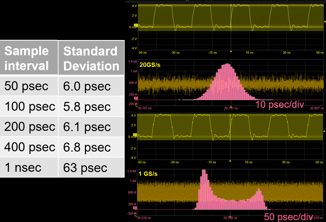
At 1 GS/s, the edges of the clock signal are not well enough defined by the number of samples to measure the period accurately. There are only about 1.3 samples on the edge (the bright dots on the zoomed clock waveform in Figure 6). As a general rule, you should use the highest possible sampling rate for jitter measurements. However, this confirms that even at a fraction of our maximum sampling rate, measurement accuracy is good, and at 20 GS/s the jitter measurement is quite trustworthy.
Copyright © 2020-2026 Teledyne LeCroy. All rights reserved. All original content, including text and photos, is the property of Teledyne LeCroy and cannot be reproduced without expressed written permission.
Want to try this with your clock source? Download our step-by-step tutorial, A Robust Method for Measuring Clock Jitter.

By correlating filtered power rail variations with clock period tracking, you can quantify and verify a clock’s jitter sensitivity to supply noise.

By injecting a controlled power rail perturbation and tracking clock period variation, you can quantify a clock’s sensitivity to supply noise.