Radar Signal Analysis With Oscilloscope Demodulation
Learn how oscilloscope demodulation and FFTs reveal radar pulse envelopes, Barker-coded phase modulation, chirp behavior, and frequency content.
Learn how oscilloscope demodulation and FFTs reveal radar pulse envelopes, Barker-coded phase modulation, chirp behavior, and frequency content.

This article explains the expected behavior of on-die power rails during CMOS switching events, including PDN current flow, clock-edge noise, and asymmetric current draw between switching and latching operations.

Learn how oscilloscope histograms help characterize component specifications by comparing propagation delay, mean, standard deviation, and measurement spread under different conditions.


A primary engineering task for 48 Volt power conversion systems using bridge topologies is to ensure adequate dead time to prevent catastrophic shoot through occurring when both HI and LO FETs conduct at the same time. Being able to accurately measure dead time is therefore of critical importance. Part 1 of this series dealt with the basic static dead time measurement. Part 2 will deal with studying the dynamic changes in the dead time measurement using statistics, tracks and histograms.
As we learned in part 1, the dead time delay is measured using two instances of the measurement parameter Delta Time at Level (dt@lvl) as shown in Figure 1.
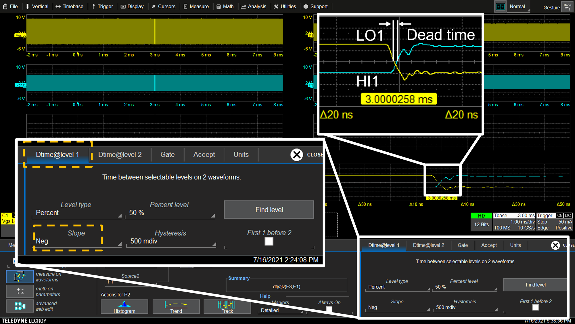
In the Figure 1, the dtime@level parameters is automating the measurement of dead times in a single acquisition with thousands of half-bridge switching transitions.
Two different measurement parameters were used to measure the two different rising/falling edge pair transitions. Only a single value is shown in Figure 2 (all values are measured, just not displayed in this instance), and the value shown is last value in the full acquisition. You should ask the question: how do the measurements vary with time?
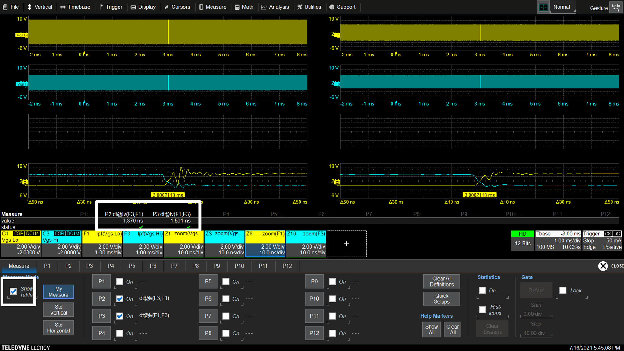
To find the answer, turn on the measurement parameter statistics, as shown in Figure 3.
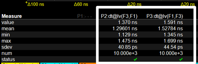
P2 and P3 have each collected 10,000 values of dead-times during the 10 ms acquisition, and the statistical table shows the last value, mean, minimum, maximum, standard deviation and number of values reported. The minimum values of both parameters are positive, indicating that shoot though has not occurred. However, this presents is very incomplete picture of the dead-time variation over time – for that we would use a Track function, or a plot of measurement values over time, time synchronized and time correlated to the original acquisition.
Figure 4 shows the track of a frequency measurement taken from another test, for purpose of illustration. Frequency decreases from ~1 MHz to ~956 kHz in eight steps corresponding to the cycles of the source waveform, which are clearly visible on the track.
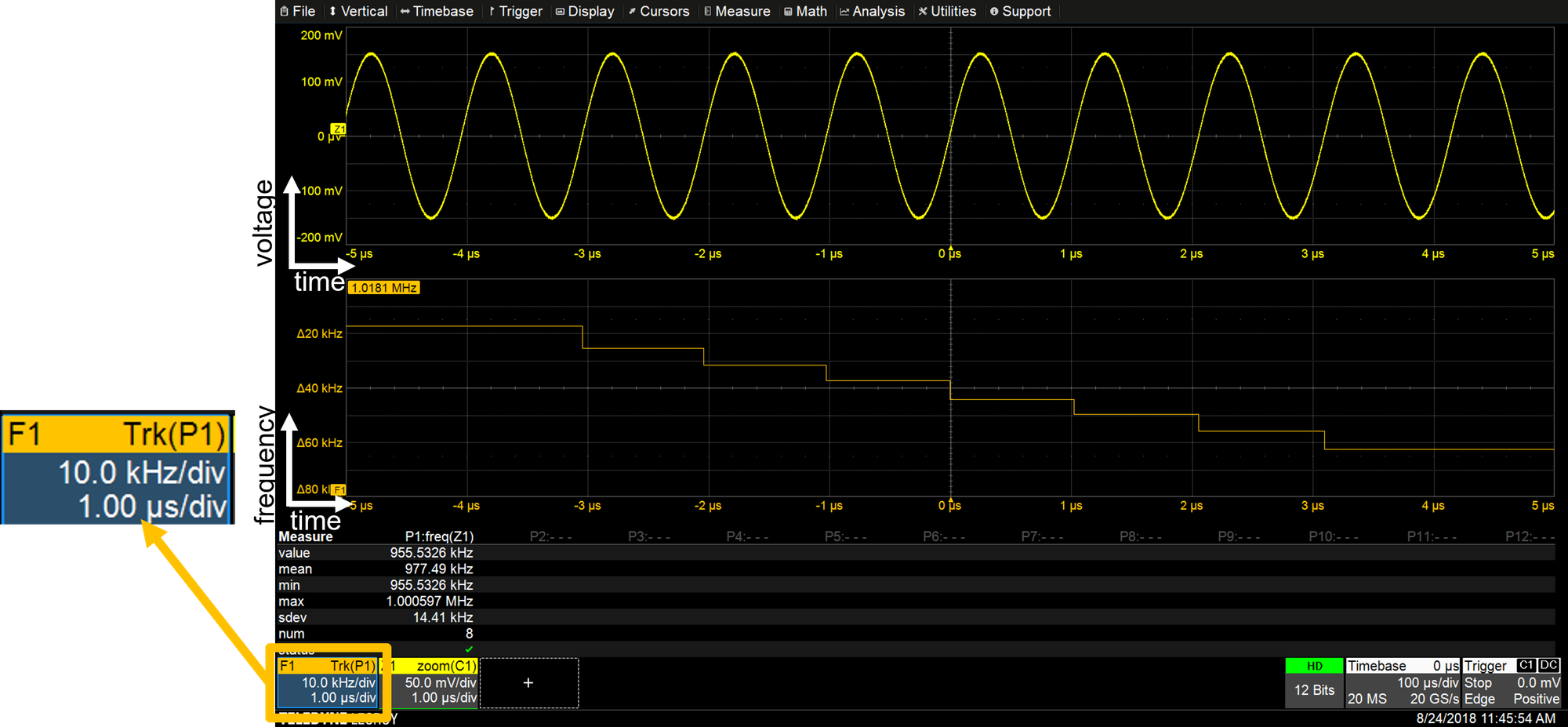
Figure 5 shows the same technique – a Track function – used to display the the two dt@lvl (dead time) parameter measurements varying in time, shown in Figure 5 (orange trace and red trace).
The track view confirms graphically that there are no delay values that are negative. Each value in a track matches up with its source on the VgsLo or VgsHi waveform. This allows any anomalous events seen on the track to be matched to the source for analysis.
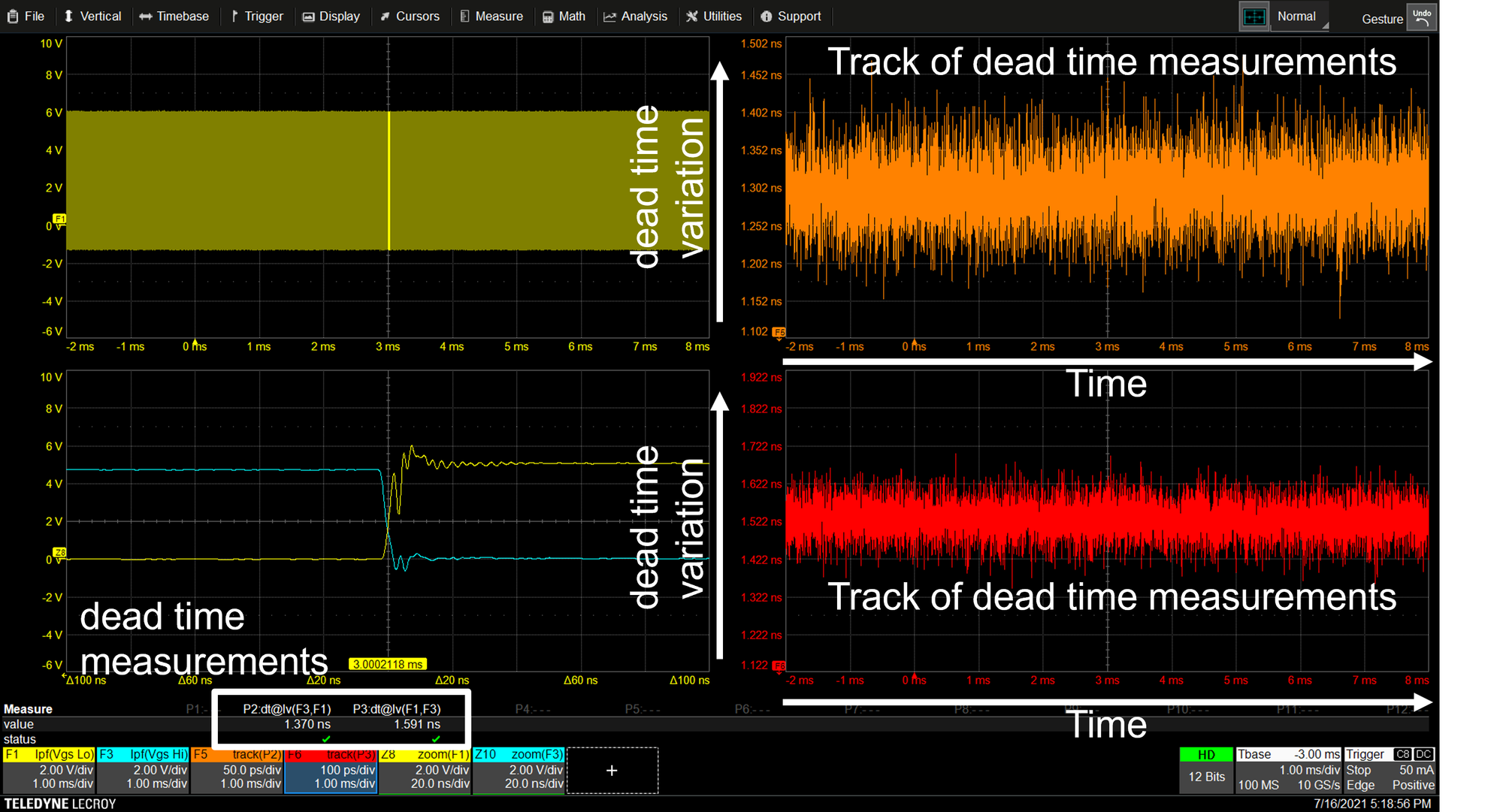
Tracks can be measured just with cursors, measurement parameters, and other tools just like any other waveform. Histograms can also be used to view the distribution of the statistical data set.
Copyright © 2020-2026 Teledyne LeCroy. All rights reserved. All original content, including text and photos, is the property of Teledyne LeCroy and cannot be reproduced without expressed written permission.
Also read the blog post Oscilloscope Basics: When to Use Track to Graph Oscilloscope Measurements