Radar Signal Analysis With Oscilloscope Demodulation
Learn how oscilloscope demodulation and FFTs reveal radar pulse envelopes, Barker-coded phase modulation, chirp behavior, and frequency content.
Learn how oscilloscope demodulation and FFTs reveal radar pulse envelopes, Barker-coded phase modulation, chirp behavior, and frequency content.

This article explains the expected behavior of on-die power rails during CMOS switching events, including PDN current flow, clock-edge noise, and asymmetric current draw between switching and latching operations.

Learn how oscilloscope histograms help characterize component specifications by comparing propagation delay, mean, standard deviation, and measurement spread under different conditions.

Learn how oscilloscope histograms help characterize component specifications by comparing propagation delay, mean, standard deviation, and measurement spread under different conditions.

In Part 1 of this series, we looked at some of the basics of histograms and how they can provide a statistical view into random variation of signal parameters. Next, let's look at how histograms can help us use statistical analysis to determine product specifications.
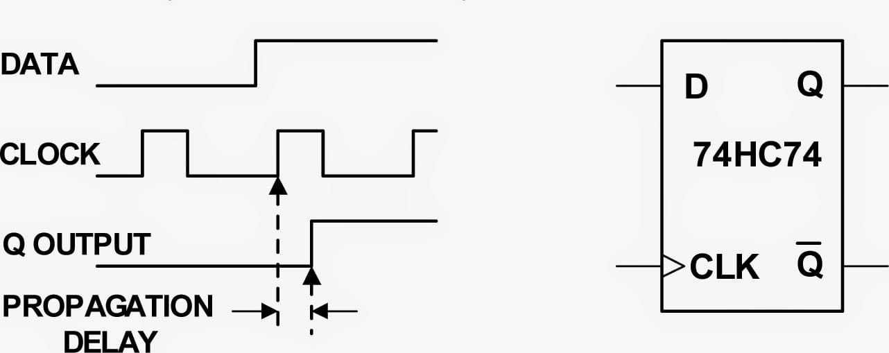
Many of Teledyne LeCroy's oscilloscopes are able to create statistical-analysis histograms on a very large number of measurements. The resulting data can be displayed as histograms (a graphical view of the data distribution), as trend plots (measurements plotted in the order taken, not time correlated to the current oscilloscope acquisition), or as track plots (measurements vs. time, time correlated to the current oscilloscope acquisition). As a result, the analysis capabilities of these instruments is extended to cover accurate readouts of up to 20 key statistical measurements such as mean, standard deviation, range, and many more.
One way to use these capabilities of an oscilloscope is to characterize the specifications of a component. Suppose you needed to verify the propagation delay of a D-type flip flop at both room temperature and at 0°C. Figure 1 shows the setup while Figure 2 depicts a propagation-delay measurement performed at room temperature.
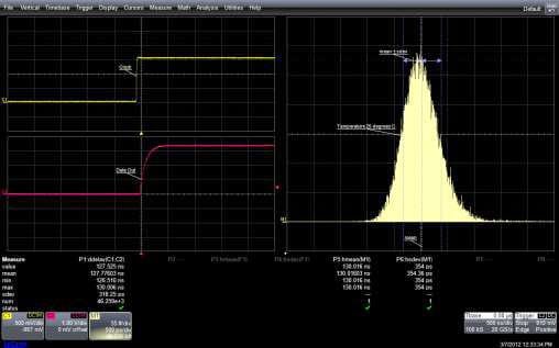
In Figure 2, the upper left-hand trace (Ch1) is the clock. Below that is the Q output (Ch2), while the right-hand trace (M1) is the histogram of the delay between positive-going edges of the clock and the Q output. The histogram shows the distribution of over 46,000 individual measurements. Meanwhile, the statistical parameters, histogram mean, and histogram standard deviation, displayed below the waveform display, provide a quantitative measure of the histogram itself. This data can be stored for later comparison when the exercise is repeated at 0°C.
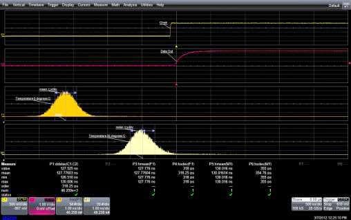
The next set of measurements, taken at 0°C, appears in Figure 3. Trace M1 contains the data taken at 25°C earlier. Trace F1, which appears above trace M1, shows that the propagation delay taken at 0°C has shifted to a lower value. The average value, or mean, has shifted from 130 ns to 127.7 ns as shown in the statistical parameter readings. In addition, the shape of the distribution has narrowed as indicated by the decrease in standard deviation from 355 to 318 ps. This shows a reduction in the spread of the measurement values. These represent only two of the possible choices for the analysis of parameter values (see below for a complete list).
This type of component characterization is quite useful in cases where the component manufacturer has not characterized the device under specific conditions required by a given application. Moreover, you have the ability to display and compare data taken at different times and under different conditions.
Besides the numerical measurement statistics provided for a typical measurement data set (mean, minimum, maximum, standard deviation and number of measurements), the histogram distribution itself may also be quantified with the following list of histogram parameters available on most Teledyne LeCroy oscilloscopes:
These measurements on the histogram itself can provide additional quantifiable context of measured behaviors that is not possible with more simplistic statistical data measurements.
Copyright © 2020-2026 Teledyne LeCroy. All rights reserved. All original content, including text and photos, is the property of Teledyne LeCroy and cannot be reproduced without expressed written permission.

Learn how oscilloscope histograms visualize measurement variation, identify distribution shapes, and quantify rare events in waveform timing and amplitude data.

This article explains how the oscilloscope Trend function differs from Track, and how it can be used for long-term measurement analysis, data logging, and monitoring evolving signal behavior across multiple acquisitions.

This article explains how the oscilloscope Track function can be used for anomaly detection and waveform demodulation by graphing synchronized measurement values directly against the input waveform.

This article explains how oscilloscope Track functions can demodulate frequency- and phase-modulated RF signals by graphing instantaneous Frequency and TIE measurements over time.