Radar Signal Analysis With Oscilloscope Demodulation
Learn how oscilloscope demodulation and FFTs reveal radar pulse envelopes, Barker-coded phase modulation, chirp behavior, and frequency content.
Learn how oscilloscope demodulation and FFTs reveal radar pulse envelopes, Barker-coded phase modulation, chirp behavior, and frequency content.

This article explains the expected behavior of on-die power rails during CMOS switching events, including PDN current flow, clock-edge noise, and asymmetric current draw between switching and latching operations.

Learn how oscilloscope histograms help characterize component specifications by comparing propagation delay, mean, standard deviation, and measurement spread under different conditions.

This article explains how oscilloscope Track functions can demodulate frequency- and phase-modulated RF signals by graphing instantaneous Frequency and TIE measurements over time.

If you are involved in RF measurements, you will eventually need to demodulate a signal. Angle modulation of either phase or frequency are the most commonly encountered modulation types. The Frequency measurement is an all-instance timing parameter that measures the frequency of every cycle in an acquired waveform. Similarly, Time Interval Error (TIE) measures the instantaneous phase of a signal on a cycle-by-cycle basis. Track functions of these measurements, which plot the values of the measurement parameter versus time, are useful for demodulating frequency and phase modulated signals, as shown in the examples below.
The track of Frequency can be used to demodulate a frequency modulated waveform. Consider a radar pulse that uses a frequency modulated ‘chirp’, as shown in Figure 1 (above).
The radio frequency carrier of the radar pulse (yellow trace top grid) has a mean frequency of 1 GHz, and it is frequency modulated by a linear ramp in frequency. Taking the Fast Fourier Transform (FFT) of this signal (blue trace second grid from top) shows that the peak amplitude response is flat, and the range of the sweep is roughly 3 MHz on either side of the 1 GHz carrier frequency. The Frequency measurement set up in parameter P1 reads the frequency of each cycle in the acquired waveform. Measurement gates are used to restrict the measurement to the region of the actual pulse burst, from roughly 2.5 to 7.5 divisions (0 to 10 ms).
A track of the Frequency measurement P1 is set up in math function F1 (gold trace third grid from top). Note the vertical axis of the track function is in units of frequency. Keep in mind that each microsecond shown on the display contains one thousand cycles of the carrier. The minor variations of frequency from cycle-to-cycle result in the noise that is evident. Math trace F5 is used to apply a low-pass filter to the track function in F1. The cutoff frequency of the Finite Impulse Response (FIR) low-pass filter is 10 kHz, and it reduces the noise significantly (orange trace bottom grid).
Parameter P2 measures the Minimum value of the filtered F5 function trace, 996.9 MHz, and likewise parameter P3 measures its Maximum value at 1.003 GHz. Parameter math set up in P4 is used to take the difference of P2 and P3, and it reports a 6.3 MHz range of frequency variation. Thus, the track of Frequency parameter P1, when suitably filtered, demodulates the frequency modulation of the radar chirp.
Demodulating a phase modulated signal can be done using a track of the TIE measurement, as shown in Figure 2.
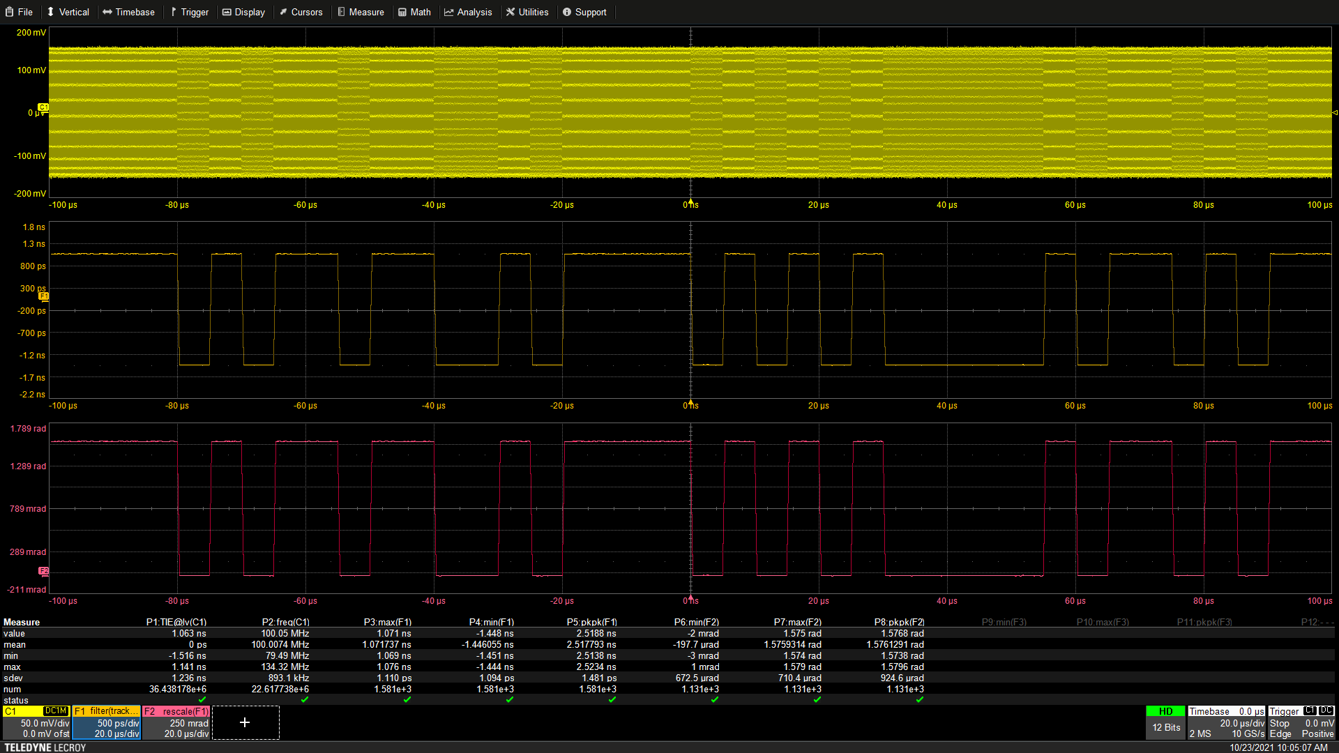
The signal acquired in channel 1 (C1) is a phase shift keyed (PSK) signal (yellow trace top grid). The carrier frequency is 100 MHz. The TIE measurement is set up in parameter P1. TIE measures the time difference between the edge of the acquired signal and the ideal edge based on the carrier frequency. The value is calculated for each cycle and is essentially the instantaneous phase of the acquired signal.
A track of TIE is set up in math function F1 (gold trace in center grid). The vertical axis is the edge delay in seconds plotted against time. At this point, the digital states of the PSK signal have been demodulated and displayed.
The Rescale math function is then used to convert time delay measurements into radians at the 100 MHz carrier frequency. Each TIE parameter value is multiplied by 628x10⁶, and the units are overridden from seconds to radians (RAD). The result is shown in F2 (magenta trace bottom grid), where the vertical units are now radians. The two binary states for this PSK signal correspond to 0 radians and 1.57 (𝜋/2) radians.
Copyright © 2020-2026 Teledyne LeCroy. All rights reserved. All original content, including text and photos, is the property of Teledyne LeCroy and cannot be reproduced without expressed written permission.

Learn how oscilloscope histograms help characterize component specifications by comparing propagation delay, mean, standard deviation, and measurement spread under different conditions.

Learn how oscilloscope histograms visualize measurement variation, identify distribution shapes, and quantify rare events in waveform timing and amplitude data.

This article explains how the oscilloscope Trend function differs from Track, and how it can be used for long-term measurement analysis, data logging, and monitoring evolving signal behavior across multiple acquisitions.

This article explains how the oscilloscope Track function can be used for anomaly detection and waveform demodulation by graphing synchronized measurement values directly against the input waveform.