Power Calculations for Distorted Waveforms

Our last post covered basic power calculations for pure sine waves, which are useful only up to a point in that pure sine waves are rather rare in the real world. Almost any real-world waveform carries some amount of distortion. Because distorted voltage and current waveforms comprise multiple frequencies, the relatively simple techniques used to measure power for pure, single-frequency sine waves no longer apply.

Among the best-known examples of a distorted waveform is a pulse-width-modulated (PWM) waveform from a motor-drive or inverter output. So that's what we'll use for examples as we look over these power calculations for distorted waveforms.

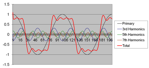
As noted above, any distorted waveform can be viewed as a collection of many sinusoids of different amplitudes and frequencies. The pseudo-square wave seen in Figure 1 has an AC fundamental augmented by a number of odd-integer harmonics. The phase relationships between voltage and current waveforms for different harmonic orders is not a constant. Thus, there's no practical method to measure phase angle between a voltage and current signal to calculate real power from apparent power. We must turn to a different approach.

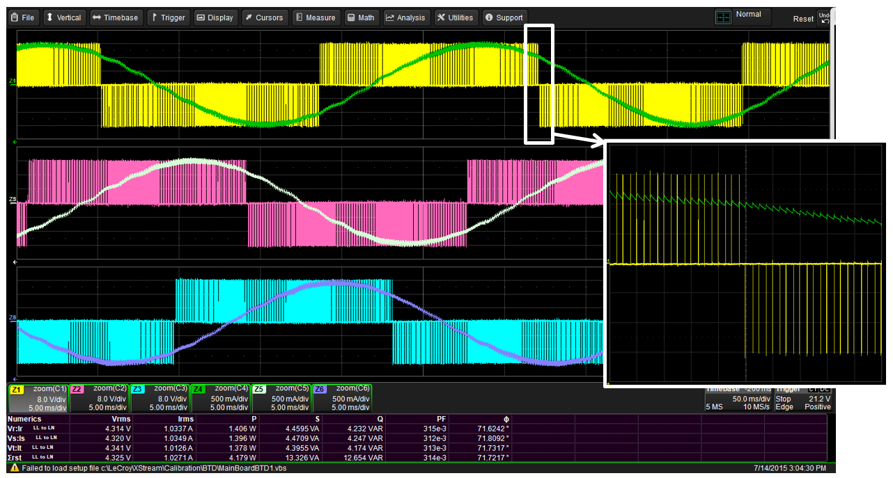
As an example, Figure 2 depicts the output waveform from a permanent-magnet, synchronous motor (PMSM) drive. Even though the line-current waveform in this three-phase signal looks sinusoidal, a closer look (inset) reveals sawtooth shapes. During overload conditions, what seems to be a decent waveform can get a lot worse; even the PWM envelope can begin to appear distorted.

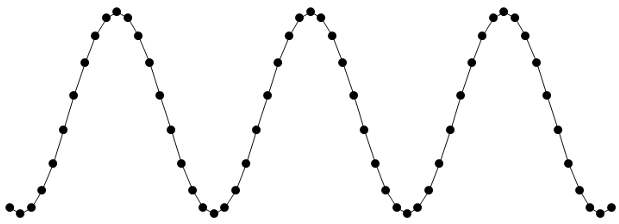
The way to handle power calculations for these sorts of distorted waveforms is with digital sampling techniques (Figure 3). An oscilloscope acquires the analog signal through sampling at a given rate and represents the signal as a collection of sampled points that are joined together by an algorithm. The result appears on the oscilloscope display as the waveform, and from there we can apply any number of math processes to the waveform to obtain power information.

The first math process to apply to the acquired and sampled signal is to determine its period, because we'll want to make one measurement per cycle. We first must choose either the current or voltage signal, whichever is closest to sinusoidal, and use that signal to define our measurement period. Our chosen signal becomes our reference, or "sync" signal.

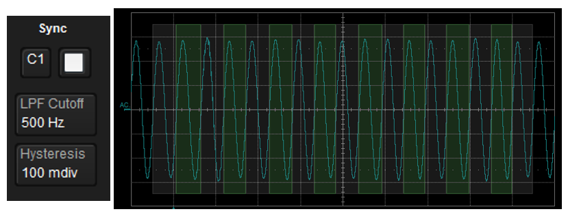
Next, we want to apply a low-pass filter to the sync signal and set a hysteresis band, and a software algorithm in the oscilloscope determines a zero-crossing point while ignoring any crossings that occur within the hysteresis band. Now we have determined a measurement period. We can slice the signal at all of the zero-crossing points into some number of measurement periods. The oscilloscope applies a highlighted overlay on top of the display grid to confirm that we have correctly established the measurement period (Figure 4). This is critical because we need to make our subsequent power calculations over a single measurement period and not over multiple periods.

Now that we've established the measurement period, we can group all the sample points into their respective measurement periods (cycles) as determined by the sync signal. For example, Figure 5 shows a signal with its sample points divided into Periods 1 and 2. In this case, Period 1 begins at sample point 7 and concludes with sample point 24, while Period 2 begins with sample point 25 and concludes with sample point 42. The example shows an identical number of sample points in both periods (18), but that's not required. In fact, if the drive is changing the frequency dynamically, there will be different numbers of sample points in each period. No matter, the algorithms that will calculate power, voltage, and current from these sample points still apply.

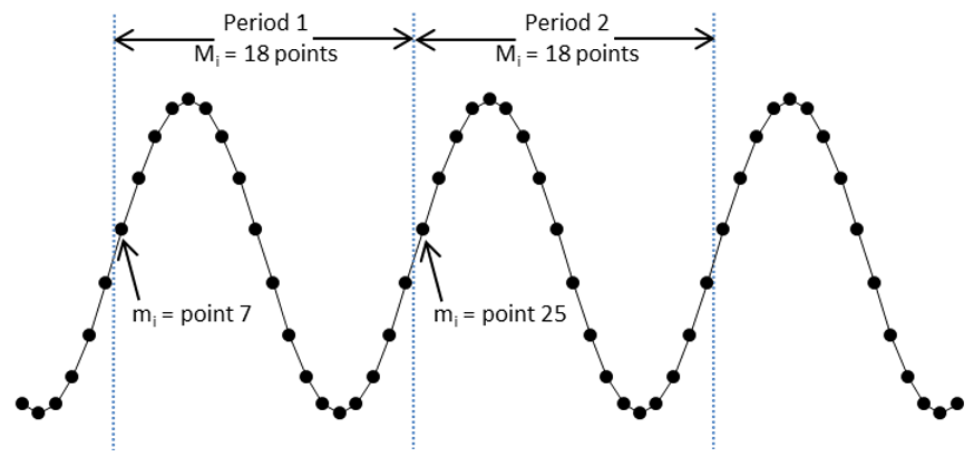
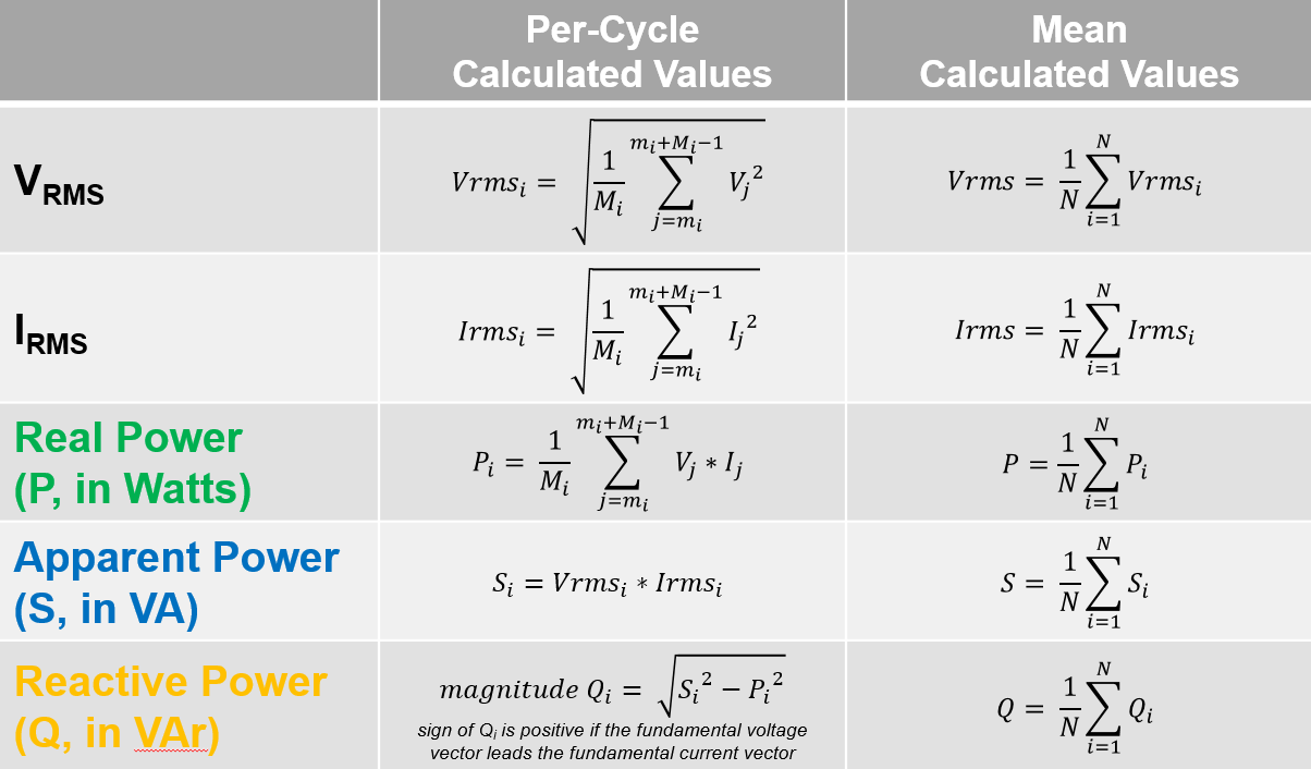
Table 1 shows the formulas used for per-cycle, digitally sampled calculations, with mean values calculated from the per-cycle data set. The criteria for the calculations are that i = measurement period (1... n, with n being the maximum number that you have). The set of waveform sample points is denoted by j. For all of the voltage, current, and power calculations, we can calculate a mean value and display those in a table, which is what a power analyzer does.

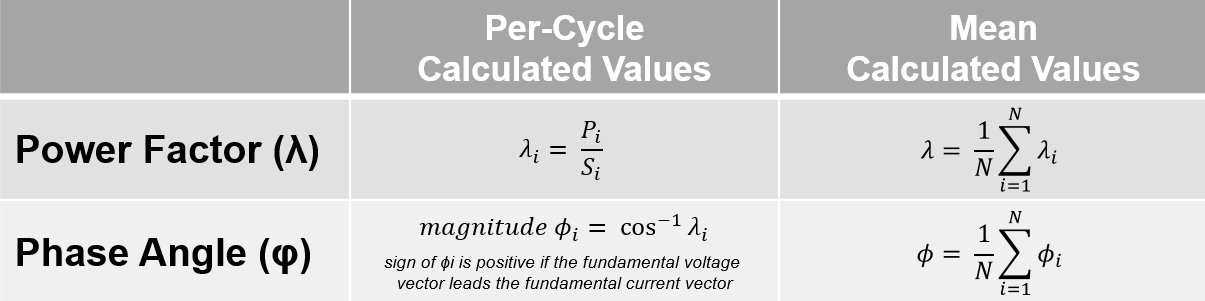
Likewise, Table 2 shows the formulas for power factor (the ratio of real to apparent power) and phase angle (the inverse cosine of the power factor).

So to sum up, the textbook descriptions of power calculations typically assume sinusoidal waveforms for single-phase systems (one voltage and one current). But the output of a power electronics converter/inverter is a distorted waveform that requires calculation methodologies that may be unfamiliar to most engineers. There's no practical way to measure phase angle between distorted voltage and current waveforms, so the only alternative is digital sampling techniques as described here (which also work for pure sine waves).

Copyright © 2020-2026 Teledyne LeCroy. All rights reserved. All original content, including text and photos, is the property of Teledyne LeCroy and cannot be reproduced without expressed written permission.