Fast Fourier Transforms on Oscilloscopes: A Hands-On Guide

Perhaps you're old enough to remember when more cars had stickshifts. They're a little bit more work to drive than cars with automatic transmissions, but the experience can be much more rewarding. Oscilloscopes these days are like cars with both types of transmissions, and you can use either one for many tasks. One of those tasks is fast Fourier transforms (FFTs), and in this post we'll take you through driving an oscilloscope to perform an FFT with a stickshift.

Figure 1 shows the time-domain view of a 50-kHz sine wave at upper left. The horizontal timebase is set at 100 μs/division, giving us 1 ms full scale. If we take 1/acquisition window, that gives us a frequency resolution of 1 kHz. Thus, the first harmonic in this signal will be at 1 kHz. The Timebase descriptor box at bottom right tells us that the sampling rate is 10 GS/s, which means that we can range up to 5 GHz in the frequency domain.

With all Teledyne LeCroy oscilloscopes that offer the MAUI UI, turning on the
FFT math function is a relatively simple matter using the Math dropdown menu. Figure 1 shows the resulting frequency-domain view of the sine wave at upper right. As we would expect, we see a peak at 50 kHz at the low end and 5 GHz as the highest frequency range.

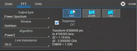
In setting up the FFT function, we remained mindful of two assumptions about FFTs. For one, it's important to set up the data truncation, and for another, to choose the windowing function (Figure 2). For the former, we're measuring 10 million data points and transforming that into 8,383,000 data points using a number from 2 to the Nth power. For the latter, the windowing function is set as the vonHann function.

From Figure 1, it's plain that most of the useful information in this FFT is at the low end of the spectrum. In Figure 3, we've zoomed in to display the FFT function at 100 kHz/division with the center frequency set at 500 kHz. Note that we are still sampling our input signal at 10 GS/s with 100-μs resolution.

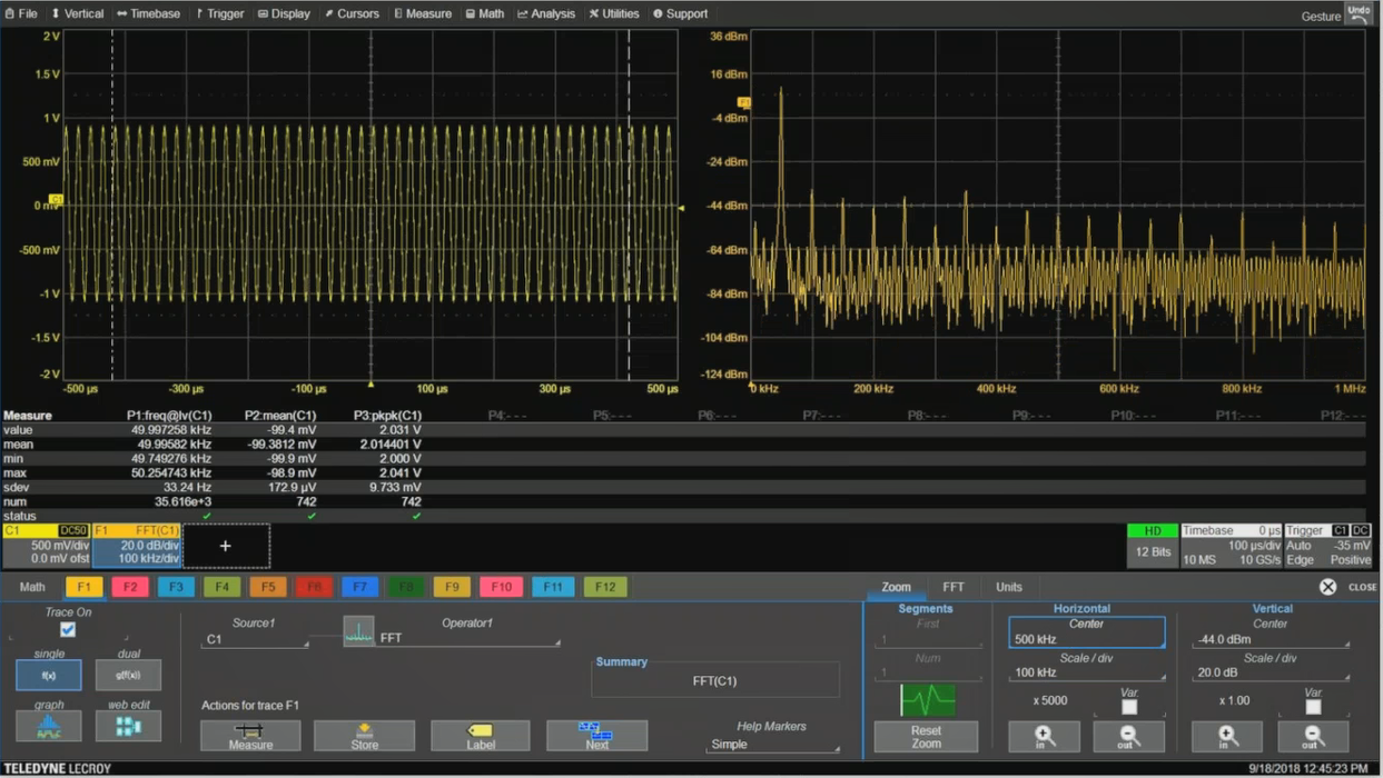
Figure 3 exposes a sharp peak at about 50 kHz with an array of subharmonics of varying amplitude at every 50 kHz interval thereafter. What looks like a clean sine wave in the time domain has been revealed to be rather distorted after all. But the signal's coming from a $13 function generator, so as with everything else in life, you get what you pay for.

That's how to perform an FFT using the oscilloscope with a manual transmission. It's more than worthwhile to learn to drive the instrument in this fashion, because in the process of setting things up you can learn a lot about what's actually going on with your signal.

Copyright © 2020-2026 Teledyne LeCroy. All rights reserved. All original content, including text and photos, is the property of Teledyne LeCroy and cannot be reproduced without expressed written permission.