Radar Signal Analysis With Oscilloscope Demodulation
Learn how oscilloscope demodulation and FFTs reveal radar pulse envelopes, Barker-coded phase modulation, chirp behavior, and frequency content.
Learn how oscilloscope demodulation and FFTs reveal radar pulse envelopes, Barker-coded phase modulation, chirp behavior, and frequency content.

This article explains the expected behavior of on-die power rails during CMOS switching events, including PDN current flow, clock-edge noise, and asymmetric current draw between switching and latching operations.

Learn how oscilloscope histograms help characterize component specifications by comparing propagation delay, mean, standard deviation, and measurement spread under different conditions.

This article explains how to properly configure an oscilloscope for EFT testing, covering sample rates, parameter acceptance, EMC pulse measurements, energy calculations, and efficient burst acquisition techniques.

A third type of electromagnetic compatibility (EMC) testing deals with how devices respond to electrical fast transients (EFT). EFTs are a series of fast, high frequency pulses, often occurring in bursts. These transient events are the result of electrical arcing. EFT pulse bursts occur when a power connection is made or broken, equipment is powered down or circuit breakers are switched. They also occur when inductive loads such as relays, switch contactors or heavy-duty motors produce bursts of narrow high-frequency transients on the power distribution system when de-energized.
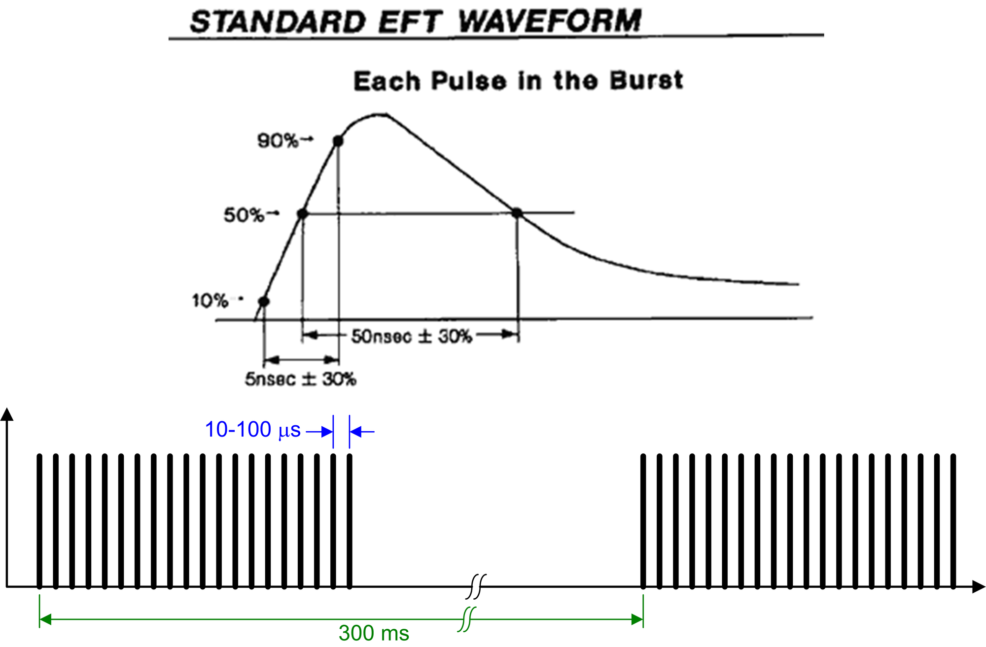
The typical compound waveform used for EFT testing is shown in Figure 1.
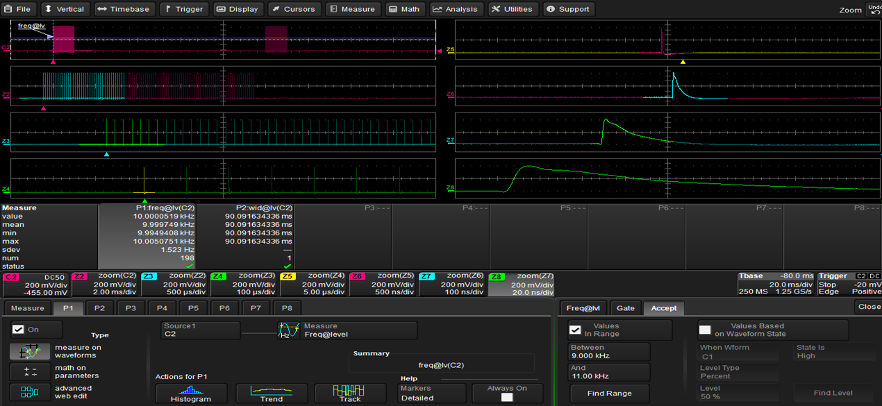
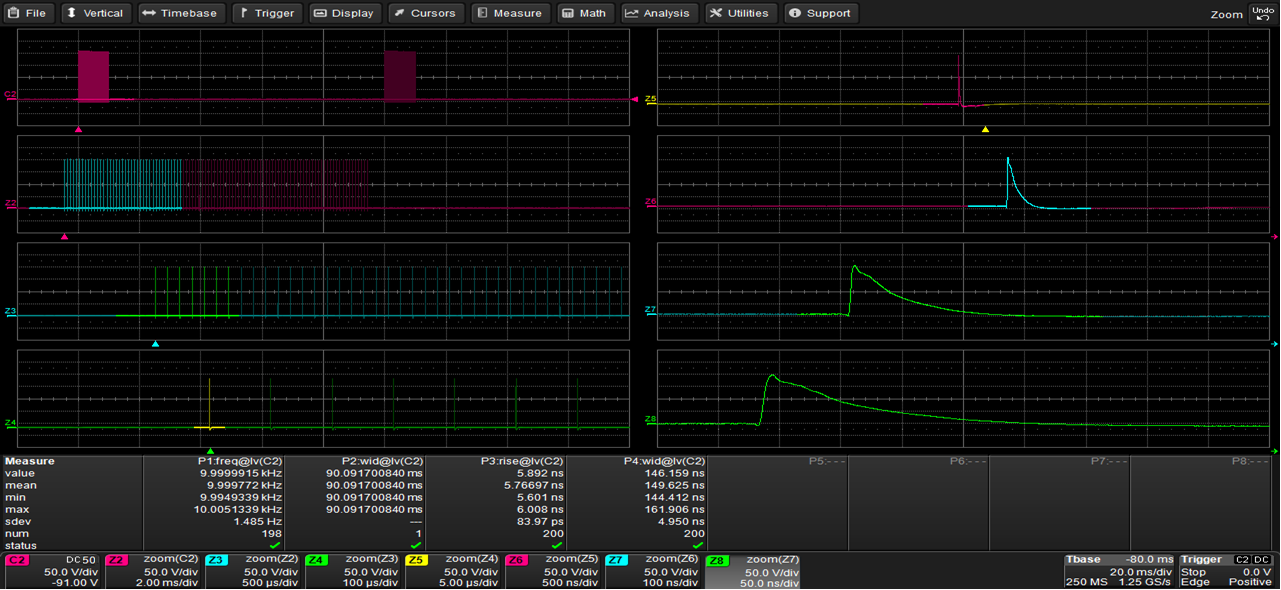
The pulse waveform for EFT testing is defined by a risetime of 5 ns and a pulse width of 50 ns. These pulses are combined into bursts of 5 to 50 pulses spaced at from 10 to 100 µs (10 to 100 kHz). The bursts are typically spaced as much as 300 ms apart. Figure 2 shows an EFT test signal, with two EFT bursts captured by an oscilloscope on channel 2 sampled at 1.25 GS/s.
The two EFT pulse burst are shown in the upper left-hand trace (the two pink blocks). A series of zoom-on-zoom traces are opened to show several timing epochs. Trace Z2 (second from top left) shows a single burst. The zooms keep expanding the horizontal scale until finally at Z8 (bottom right) we see a single EFT pulse.
Following are six, important things to do to make sure you get the best EFT test measurements from your oscilloscope.
Given the fast rise time of the EFT pulse, the oscilloscope’s sample rate should be high enough to characterize the fast edge and to guarantee that the peaks are adequately sampled. For the examples shown here, the sample rate was set to 1.25 GS/s. This assures over six samples on the fast edge and a good characterization of the peaks of the waveform.
One measurement of interest is the pulse repetition rate within the burst. The frequency parameter can be used to make this measurement, but because the source waveform (C2) is a burst waveform, it will show the pulse repetition rate along with the burst repetition rate. To look at only the higher frequency pulse repetition rate, use parameter acceptance to report only measured values that fall within a user-defined range. Figure 2 shows the Accept subdialog set up for a range of 9 to 11 kHz. Parameter P1 shows the corrected measurement of 10 kHz.
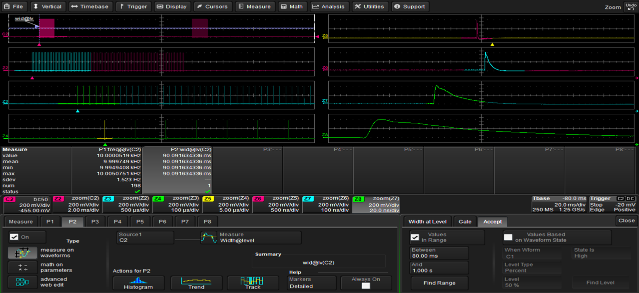
It is often asked, "how do you measure the gap time in between the bursts of EFT pulses?" You could simply measure negative pulse width (between a falling and a rising edge), but then you'd get the negative pulse width between each of those individual EFT pulses, not just the inter-burst gaps. Again, this is a case for using parameter acceptance, as shown in parameter P2 of Figure 3. Set up a pulse Width @ Level parameter with a negative polarity, then accept the lowest and highest measurement values that potentially define the inter-burst gaps. In this example, the limits of 80 milliseconds and 1 second exclude those individual high-frequency pulse widths, only measuring the gap time in between EFT bursts.
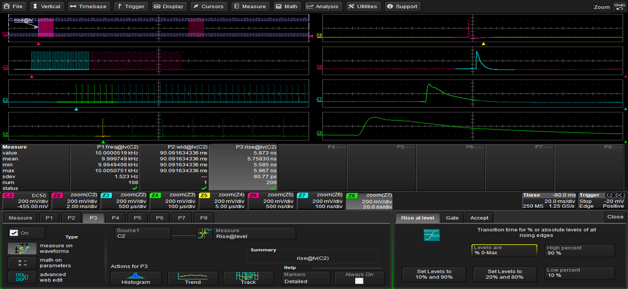
Other typical EFT measurement are the rise time and width of the individual pulses. As with other types of EMC test waveforms that are not bi-level and therefore do not have a top and base, non-rectangular EFT pulses require that measurements be made using the % 0 - Max amplitude reference level, as shown in Figure 4.
Some EFT standards require the measurement of pulse maximum amplitude, pulse area and energy.
To calculate energy, follow these steps (Figure 5):
The energy of our EFT pulse is automatically calculated at 7.35 micro-Joules.
The waveforms acquired for EFT measurements can have very small duty cycles, being short pulses separated by long intervals with no activity. This type of waveform can use up a lot of oscilloscope memory. One way to extend memory is to use sequence mode acquisition. Sequence mode captures smaller segments of interest (of a user-defined length) based on a triggering event. Once triggered, the oscilloscope only acquires data for the duration of the interesting activity, storing one segment in memory, then stops acquiring until the next trigger. Figure 6 shows an EFT acquisition made for ISO 7637 that uses sequence mode.
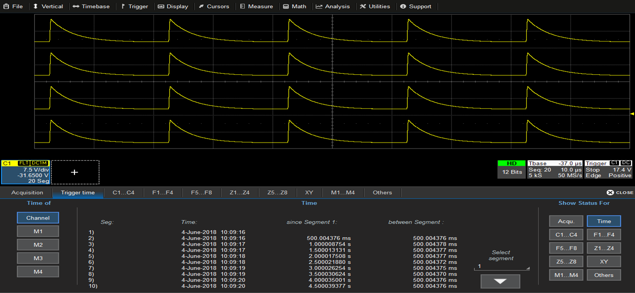
The event of interest is a narrow pulse (15 µs width), followed by an electrical idle for the balance of the 500 ms period, representing a duty cycle of only 0.003%. By using sequence mode with a trigger set on the 15 µs width, you can capture 20 segments at 50 MS/s using only 5000 samples per segment, a total of only 100,000 samples, instead of the 50 million samples it would take to capture 10 such pulses using real-time sampling mode.

This article explains how to properly configure an oscilloscope for ESD pulse testing, covering rise-time thresholds, EMC pulse measurements, parameter limiting, and automated trend capture for compliance testing.

This article explains how to properly configure an oscilloscope for surge testing, including attenuation setup, measurement threshold adjustments, and calculating pulse area and transferred charge.

Accurate ESD pulse measurement depends on using a high enough sampling rate to capture sufficient points on the rising edge for reliable characterization.

Standard IEEE pulse definitions can misinterpret fast-decaying ESD pulses, requiring manual threshold adjustments for accurate measurements.