Radar Signal Analysis With Oscilloscope Demodulation
Learn how oscilloscope demodulation and FFTs reveal radar pulse envelopes, Barker-coded phase modulation, chirp behavior, and frequency content.
Learn how oscilloscope demodulation and FFTs reveal radar pulse envelopes, Barker-coded phase modulation, chirp behavior, and frequency content.

This article explains the expected behavior of on-die power rails during CMOS switching events, including PDN current flow, clock-edge noise, and asymmetric current draw between switching and latching operations.

Learn how oscilloscope histograms help characterize component specifications by comparing propagation delay, mean, standard deviation, and measurement spread under different conditions.

This article explains how to properly configure an oscilloscope for surge testing, including attenuation setup, measurement threshold adjustments, and calculating pulse area and transferred charge.

Electrical surges result from phenomena like lightning strikes and switching transients. Electronic devices are subjected to simulated surges to confirm that they continue to operate properly following a surge, just as they are tested against electrostatic discharge.
Surge pulses are similar to ESD pulses in that they have a very fast rise time, but the fall time is much, much slower. Figure 1 shows a typical surge pulse waveform. Surge testing involves similar measurements to those made for ESD pulse testing—such as rise time, pulse width and max—but surge testing also requires some additional measurements, such as area under the pulse curve and transmitted charge.
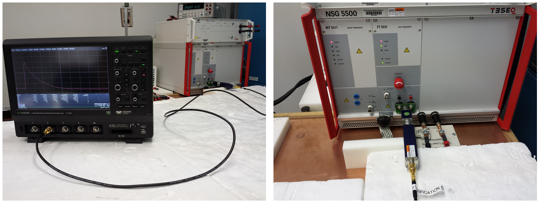
As with ESD pulse tests, oscilloscopes are primarily used to “test the tester,” confirming the output of the surge generator. So, before a surge generator is hooked up to the device under test, it's required to hook it up to an oscilloscope and conduct a series of measurements to make sure the surge pulse is within specification. Figure 2 shows a typical surge test setup.
Following are three, important things to do to make sure you get the best surge measurements from your oscilloscope.
As was the case with ESD testing, the oscilloscope is set to a 50 Ω input termination. The input to the oscilloscope from the surge generator has to be less than 5 Vrms. This means that a suitable attenuator must be inserted between the surge generator and the oscilloscope as shown in Figure 2. The attenuation ratio should entered into the Attenuation field on the oscilloscope’s input channel dialog so that the oscilloscope’s readout is calibrated to the properly scaled voltage on the screen display.
The surge pulse, like the ESD pulse, is not a rectangular pulse and should not be measured using the oscilloscope’s default measurement settings. These setting are intended for rectangular pulses with two clearly defined levels. Instead, measurements should be made using the % 0-Max reference level setting, as shown in the setup for the rise time measurement in Figure 3.
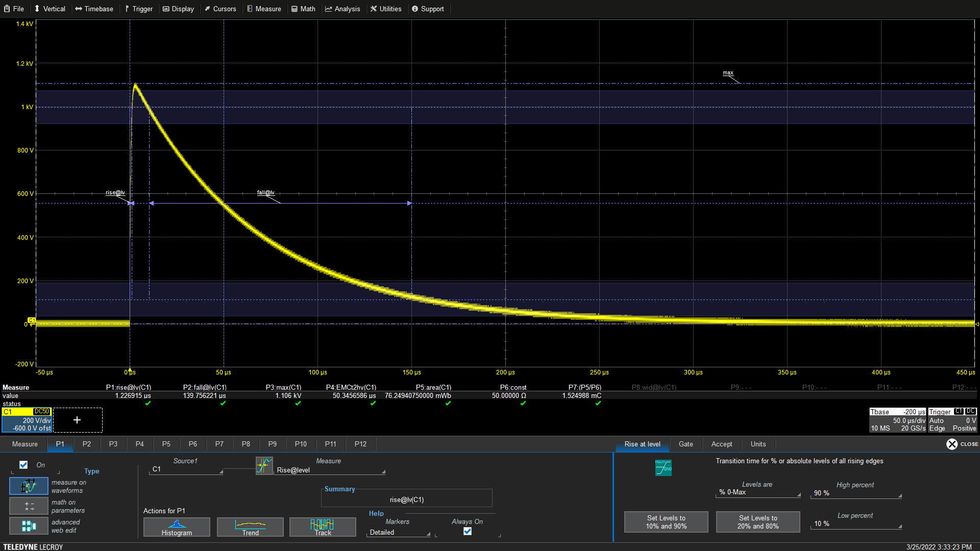
The reference levels for the rise time measurement in Figure 3 are shown as dash-dot-dot markers in blue. The high and low percent thresholds appear as dashed blue lines at the 10 and 90% levels. The rise time is about 1.2 µs while the fall time is about 140 µs and maximum voltage is 1.1 kV.
As in the case of the ESD pulse test, we used the optional EMC Pulse Parameter Time to Half Level (EMCt2hv) to measure the time from the leading edge of the pulse until the amplitude falls to half the maximum value, nominally 50 µs.
The surge standards require some measurements in addition to those made for ESD testing. The first is the area under the pulse. Area is a standard oscilloscope measurement and as the name implies uses an integral function to measure the area under the acquired pulse. The result is shown in parameter readout P5 as 76 milli-Webers (Volt-seconds).
The area measurement is then used to calculate the charge transferred by the pulse. If we divide the area by the oscilloscope’s input impedance, we get the charge in Coulombs (Ampere-seconds).
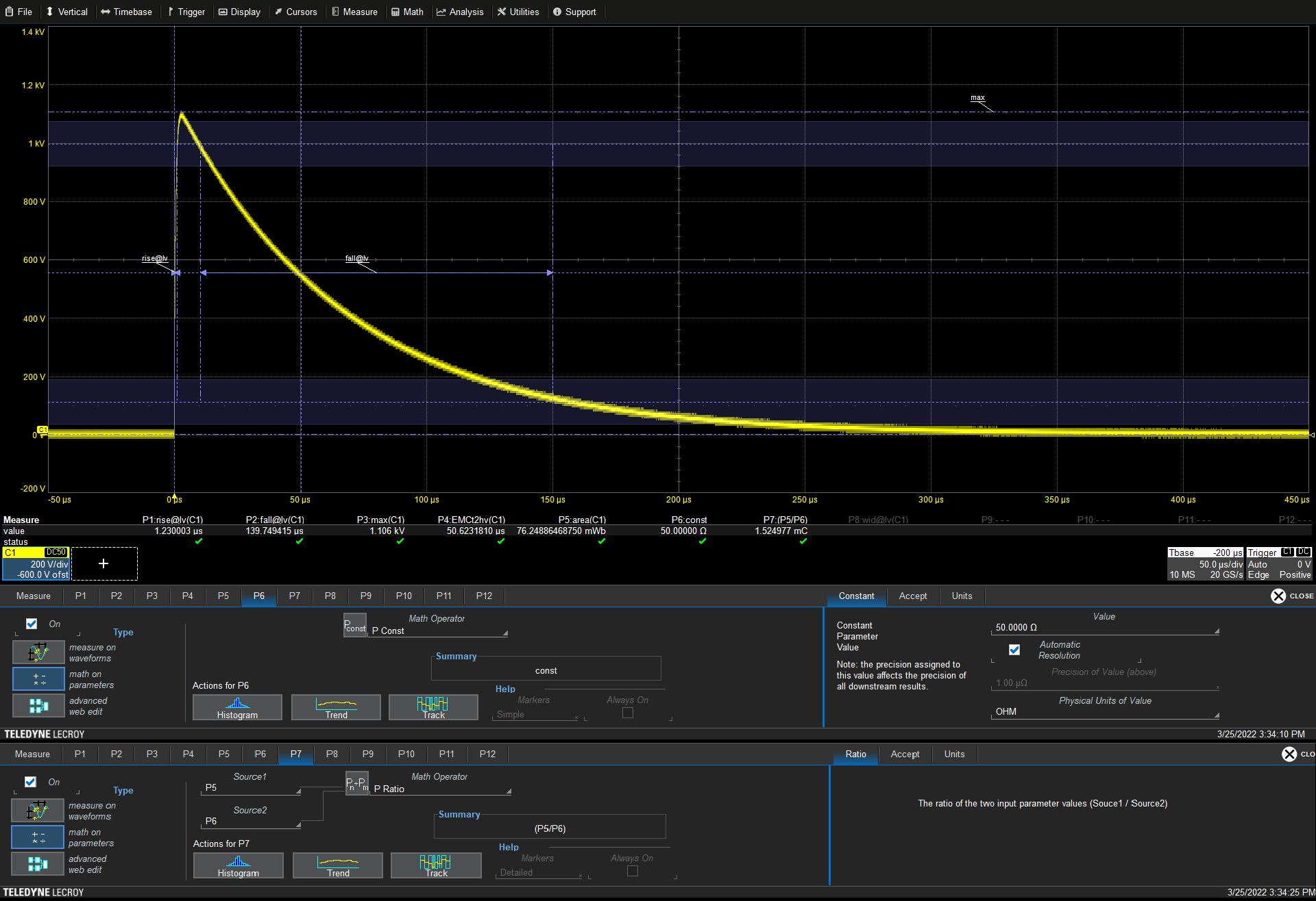
The calculation of the charge uses the oscilloscope’s Math on Parameters feature, as shown in Figure 4. Parameter P6 defines a constant using the operator P Const; in this case the constant is the 50 Ω of the oscilloscope input impedance. Note that a physical unit can be associated with the constant, in this case the unit Ohms was used.
Next, the Math on Parameters operator P Ratio is used to divide the area in P5 by the constant in P6. The oscilloscope automatically assigns the proper units, milli-Coulombs (mC), to the calculation, showing a charge of 1.5 mC.

This article explains how to properly configure an oscilloscope for ESD pulse testing, covering rise-time thresholds, EMC pulse measurements, parameter limiting, and automated trend capture for compliance testing.

This article explains how to properly configure an oscilloscope for EFT testing, covering sample rates, parameter acceptance, EMC pulse measurements, energy calculations, and efficient burst acquisition techniques.

Accurate ESD pulse measurement depends on using a high enough sampling rate to capture sufficient points on the rising edge for reliable characterization.

Standard IEEE pulse definitions can misinterpret fast-decaying ESD pulses, requiring manual threshold adjustments for accurate measurements.